Wahid - Pakistan : How to automatically find the highest three positions?
Solutions:
Yes! There are number of ways to find the highest number, I am giving you an example of the function RANK().
RANK (number, ref, order)
Number is the number whose rank you want to find.
Ref is a list of numbers.
Order “0” for Descending else for Ascending.
This function as its name says, tells you the RANK of a specific number in the list of numbers. Let’s try it.
1. Open a new excel file.
2. Write 10,20,30,40 in Cell Number A1, A2, A3 and A4 respectively
3. Select cell B1 and write “=rank(“ then move Left Arrow Key to cell A1 then press “,” and move again Left Arrow Key to cell A1 then press “Shift” key and press Down Arrow Key till cell A4. Now press “F4” key (to fix the list) then press “,” and write “0” for Descending Order, close the bracket and press “Enter”.
4. Now you will see the number “4” in cell B1 and your formula will look like “=RANK(A1,$A$1:$A$4,0)” in Formula Bar.
5. Copy Cell B1 and paste it from B2 to B4.
6. You will get the position of that specific number in the list from Highest to Lowest (Descending Order).
To automate the finding of first three positions in a Result Card you may use a combination of IF() and RANK() to perform the job. Let’s try it.
1. Continuing with the previous sheet, now in Cell C1 write “=IF(RANK(A1,$A$1:$A$4,0)>3,"",IF(RANK(A1,$A$1:$A$4,0)=1,"First",IF(RANK(A1,$A$1:$A$4,0)=2,"Second",IF(RANK(A1,$A$1:$A$4,0)=3,"Third",""))))”.
2. Copy the Cell C1 and paste it from Cell C2 to C4.
3. Congratulations! You have find the first Three Positions.
Enjoy Learning!
Shakil - India : How to create macro in excel
Dear Shakil,
You can either 'Record a macro' or 'Write a macro'. To write a macro you will need to have command over VBA however to record a Macro you don’t need any language skill.
To Record a Macro:
Open a new excel file and on Cell A1 type “Shakil”.
Click to VIEW Ribbon (menu) in Excel 2007, you will find ‘Macros’ tab in the end, Click on it and select “Record Macro” (In previous version Go to Tools->Macros->Record a Macro).
This will pop up a window asking you to choose a name and shortcut for the macro etc. Let’s give it the name “Shakil”, Shortcut key “k” (to set the shortcut to “Ctrl+k”). Click OK button.
Now Excel will record anything you do on the worksheet, do whatever you want... eg type “=IF(A1="Shakil"," is a quick learner"," is not a quick learner")” on cell B1. Press Enter.
Now go to the Macros Tab and click “stop recording”.
Congratulations! You have successfully created the Macro named “Shakil”.
Now delete all data on the sheet. Type “Shakil” on any cell on the worksheet and then move to next cell and hit “Ctrl+k”. you will be displayed the result.
Enjoy Learning!
Dilawar Abbas - Pakistan : Convert Numaric Figures into Words
Solution:
Dear Dilawar Abbas,
Microsoft Excel has various function embedded built-in but still they are not enough to provide customized solutions. The good thing is that Microsoft Excel allow to its users to create their own functions according to their desired needs but for that you should have some command in VB (Visual Basic).
Dont worry! you don't have to write VB codes on your own, I have written down TWO CODES for you both to convert Numbers into Simple Text (i.e. 115 to One Hundred Fifteen Only) and Numbers into Pak Currency (i.e. 25 to Twenty Five Rupees Only). Please follow the instructions below:
To Convert Numbers into Words:
3. On Menu Bar Click to Insert -> Module.
4. New window opens, now Copy the code given below and Paste it.
5. Close the window.
6. Save the Excel file by selecting the file type as "Macro-Enabled Workbook".
7. Congratulations! New function named "SpellNumber" with syntex "=SpellNumber(cell ref!)" has been created.
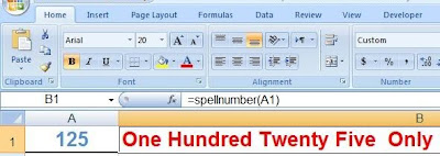
8. Now you can use the function on any cell, for example : if CELL A1 contains the number "125", on CELL B1 type "=spellnumber(A1)" and the number will be spelled as "One Hundred Twenty Five".
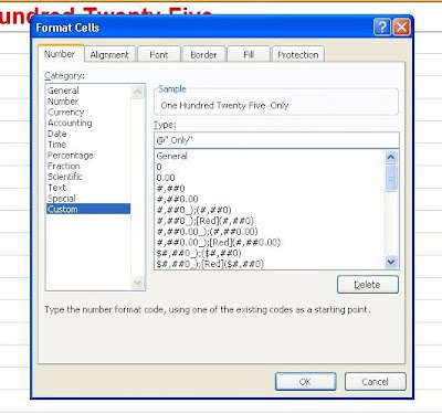
9. To add the word "Only", we'll do it by Cell Custom Formatting.
10. Right Click on the CELL B1, click "Format Cells", on the "Number" tab click on "Custom" and Under "Type" text box write [ @" Only" ] (See figures).
CODE:
Function SpellNumber(ByVal MyNumber)
Dim Rupees, Temp
Dim DecimalPlace, Count
ReDim Place(9) As String
Place(2) = " Thousand "
Place(3) = " Million "
Place(4) = " Billion "
Place(5) = " Trillion "
MyNumber = Trim(Str(MyNumber))
DecimalPlace = InStr(MyNumber, ".")
If DecimalPlace > 0 Then
Paisas = GetTens(Left(Mid(MyNumber, DecimalPlace + 1) & "00", 2)) MyNumber = Trim(Left(MyNumber, DecimalPlace - 1))
End If
Count = 1
Do While MyNumber <> ""
Temp = GetHundreds(Right(MyNumber, 3))
If Temp <> "" Then Rupees = Temp & Place(Count) & Rupees
If Len(MyNumber) > 3 Then
MyNumber = Left(MyNumber, Len(MyNumber) - 3)
Else
MyNumber = ""
End If
Count = Count + 1
Loop
Select Case Rupees
Case ""
Rupees = ""
Case "One"
Rupees = "One "
Case Else
Rupees = Rupees & " "
End Select
SpellNumber = Rupees
End Function
Function GetHundreds(ByVal MyNumber)
Dim Result As String
If Val(MyNumber) = 0 Then Exit Function
MyNumber = Right("000" & MyNumber, 3)
If Mid(MyNumber, 1, 1) <> "0" Then
Result = GetDigit(Mid(MyNumber, 1, 1)) & " Hundred "
End If
If Mid(MyNumber, 2, 1) <> "0" Then
Result = Result & GetTens(Mid(MyNumber, 2))
Else
Result = Result & GetDigit(Mid(MyNumber, 3))
End If
GetHundreds = Result
End Function
Function GetTens(TensText)
Dim Result As String
Result = ""
If Val(Left(TensText, 1)) = 1 Then
Select Case Val(TensText)
Case 10: Result = "Ten"
Case 11: Result = "Eleven"
Case 12: Result = "Twelve"
Case 13: Result = "Thirteen"
Case 14: Result = "Fourteen"
Case 15: Result = "Fifteen"
Case 16: Result = "Sixteen"
Case 17: Result = "Seventeen"
Case 18: Result = "Eighteen"
Case 19: Result = "Nineteen"
Case Else
End Select
Else
Select Case Val(Left(TensText, 1))
Case 2: Result = "Twenty "
Case 3: Result = "Thirty "
Case 4: Result = "Forty "
Case 5: Result = "Fifty "
Case 6: Result = "Sixty "
Case 7: Result = "Seventy "
Case 8: Result = "Eighty "
Case 9: Result = "Ninety "
Case Else
End Select
Result = Result & GetDigit(Right(TensText, 1))
End If
GetTens = Result
End Function
Function GetDigit(Digit)
Select Case Val(Digit)
Case 1: GetDigit = "One"
Case 2: GetDigit = "Two"
Case 3: GetDigit = "Three"
Case 4: GetDigit = "Four"
Case 5: GetDigit = "Five"
Case 6: GetDigit = "Six"
Case 7: GetDigit = "Seven"
Case 8: GetDigit = "Eight"
Case 9: GetDigit = "Nine"
Case Else: GetDigit = ""
End Select
End Function

Download Figures to Words Sample File
1. Open Excel New Workbook (File).
2. Press Alt+F11.
3. On Menu Bar Click to Insert -> Module.
4. New window opens, now Copy the code given below and Paste it.
5. Close the window.
6. Save the Excel file by selecting the file type as "Macro-Enabled Workbook".
7. Congratulations! New function named "SpellNumber" with syntex "=SpellNumber(cell ref!)" has been created.
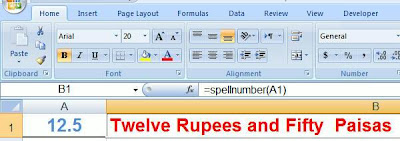
8. Now you can use the function on any cell, for example : if CELL A1 contains the number "12.5", on CELL B1 type "=spellnumber(A1)" and the number will be spelled as "Twelve Rupees and Fifty Paisas".
9. To add the word "Only", we'll do it by Cell Custom Formatting.
10. Right Click on the CELL B1, click "Format Cells", on the "Number" tab click on "Custom" and Under "Type" text box write [ @" Only" ] (See figures).

Dim Rupees, Paisas, Temp
Dim DecimalPlace, Count
ReDim Place(9) As String
Place(2) = " Thousand "
Place(3) = " Million "
Place(4) = " Billion "
Place(5) = " Trillion "
MyNumber = Trim(Str(MyNumber))
DecimalPlace = InStr(MyNumber, ".")
If DecimalPlace > 0 Then
Paisas = GetTens(Left(Mid(MyNumber, DecimalPlace + 1) & "00", 2)) MyNumber = Trim(Left(MyNumber, DecimalPlace - 1))
End If
Count = 1
Do While MyNumber <> ""
Temp = GetHundreds(Right(MyNumber, 3))
If Temp <> "" Then Rupees = Temp & Place(Count) & Rupees
If Len(MyNumber) > 3 Then
MyNumber = Left(MyNumber, Len(MyNumber) - 3)
Else
MyNumber = ""
End If
Count = Count + 1
Loop
Select Case Rupees
Case ""
Rupees = ""
Case "One"
Rupees = "One Rupee"
Case Else
Rupees = Rupees & " Rupees"
End Select
Select Case Paisas
Case ""
Paisas = ""
Case "One"
Paisas = " and One Paisa"
Case Else
Paisas = " and " & Paisas & " Paisas"
End Select
SpellNumber = Rupees & Paisas
End Function
Function GetHundreds(ByVal MyNumber)
Dim Result As String
If Val(MyNumber) = 0 Then Exit Function
MyNumber = Right("000" & MyNumber, 3)
If Mid(MyNumber, 1, 1) <> "0" Then
Result = GetDigit(Mid(MyNumber, 1, 1)) & " Hundred "
End If
If Mid(MyNumber, 2, 1) <> "0" Then
Result = Result & GetTens(Mid(MyNumber, 2))
Else
Result = Result & GetDigit(Mid(MyNumber, 3))
End If
GetHundreds = Result
End Function
Function GetTens(TensText)
Dim Result As String
Result = ""
If Val(Left(TensText, 1)) = 1 Then
Select Case Val(TensText)
Case 10: Result = "Ten"
Case 11: Result = "Eleven"
Case 12: Result = "Twelve"
Case 13: Result = "Thirteen"
Case 14: Result = "Fourteen"
Case 15: Result = "Fifteen"
Case 16: Result = "Sixteen"
Case 17: Result = "Seventeen"
Case 18: Result = "Eighteen"
Case 19: Result = "Nineteen"
Case Else
End Select
Else
Select Case Val(Left(TensText, 1))
Case 2: Result = "Twenty "
Case 3: Result = "Thirty "
Case 4: Result = "Forty "
Case 5: Result = "Fifty "
Case 6: Result = "Sixty "
Case 7: Result = "Seventy "
Case 8: Result = "Eighty "
Case 9: Result = "Ninety "
Case Else
End Select
Result = Result & GetDigit(Right(TensText, 1)) End If
GetTens = Result
End Function
Function GetDigit(Digit)
Select Case Val(Digit)
Case 1: GetDigit = "One"
Case 2: GetDigit = "Two"
Case 3: GetDigit = "Three"
Case 4: GetDigit = "Four"
Case 5: GetDigit = "Five"
Case 6: GetDigit = "Six"
Case 7: GetDigit = "Seven"
Case 8: GetDigit = "Eight"
Case 9: GetDigit = "Nine"
Case Else: GetDigit = ""
End Select
End Function

Download Figures to Currency Words Sample File
Irfan - Pakistan : VB Forms in Excel 2007
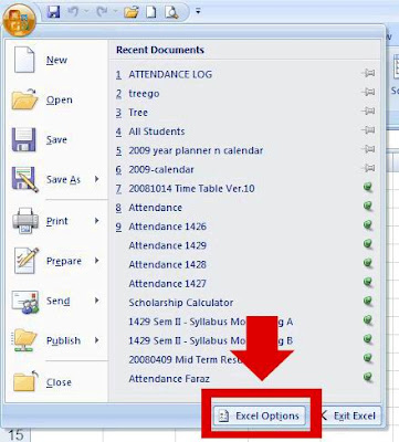
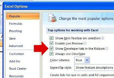
"Developer" Ribbon (where Active-x and Form Controls are available) does not appear when you install fresh Excel 2007, to activate this Ribbon you have to follow these steps.
Sheraz Ahmed - Pakistan : How to Unprotect the Protected Excel Sheets
Solution:
Dear Sheraz,
If one forgets the Password, there is no other way to unprotect the protected sheets within the Excel itself. However, i am giving a very useful TIP. Try this tip, follow the steps below, I hope your problem will be solved in minutes.
STEP 1:
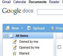
Login to Google Accounts Page : http://www.google.com/accounts and click on "DOC" or you can directly log into the Google Doc page : http://www.google.com/doc.
STEP 2:
On Menu bar Click "Upload" and browse your Excel file that have protected sheet.
Google Doc will then upload, save and open the file in new window.
Now from the "File" Menu, click to "Export" and save the file to your derired folder with your desired file name.
STEP 3:
Now open the file and your sheet will now no more password protected.
Enjoy Learning!
Azhar Hussain asked from Pakistan
I need to remove word Count from the whole list as well as want to make sure that initial 2 zeros should not be removed.
For Example.
Pls remove "Count" but make sure that first 2 zeros "00" should not be removed or deleted.
00-0004
00-0005 Count
0-001 Count
0006648-801 Count
00083-002 Count
00131-022-005 Count
0013374 Count
0013879 Count
0013888 Count
0013889-15 Count
Solution:
Dear Azhar Hussain,
You can do it easily by using the "LEFT" function available in Excel. Follow the steps below:
Step 1: click on the cell just after the first cell of the list of numbers.
Step 2: write "=LEFT(A2, LEN(A2)-5)", where "A2" is cell reference and "-5" is the number of characters you wish to erase from the field.
Step 3: copy the formula down the cells till the list ends.


